
João
Home Page


Research > Auger Physics
The main objective of the Pierre Auger Observatory is to study tthe Cosmic Rays and to answer some quastions like: what are the origin of the cosmic rays?; What are the cosmic ray composition?; What are the behavior of the hadronic interactions?; study the GZK cutoff and several others.
In this section I have include:
- Ultra High Energy Cosmic Rays (UHECR)
- Sources and anisotropies
- Extensive Air Shower (EAS)
- Hadronic Models an Particle Physics
Ultra High Energy Cosmic Rays (UHECR)
The Cosmic Ray term is somewhat misleading, since it is a radiation that consists mainly of ionized atomic nuclei. The term was assigned by Robert Millikan, after V. Hess prove it came from space. Millikan believed that throughout the universe, there was the release of binding energy of atoms in the form of gamma rays, and this would be the cosmic rays. This radiation is simply particles that collide with earth, have various compositions and a wide range of energies (see wiki for more information).

In the Figure we have the particle rate that hits our atmosphere (cosmic rays) versus evenrgy (in 1eV=1.6e^-19Joule). We can see a variation in flux of 33 orders of magnitude, for a energy range of about 15 orders(10^6eV to 10^21eV at least), note that, since the flux decrease very fast, it is multiplied by Energy^2. For example, at 10^11eV we have a rate of 1particle per m^-2s^-1, while for 10^20eV,we have about 1/km2/century.
In this way, we can detect cosmic rays with energy lower than 10^14/10^15eV (with balloons and satellites). However, for higher energies, we have so few particles that we would need huge areas of detection. So is obvious that it will not be possible to directly detect those particle with one detector. Therefore, we use the atmosphere as a detector (calorimeter) and cosmic rays are detected in the atmosphere as cascades of particles (which will be described in the next section).
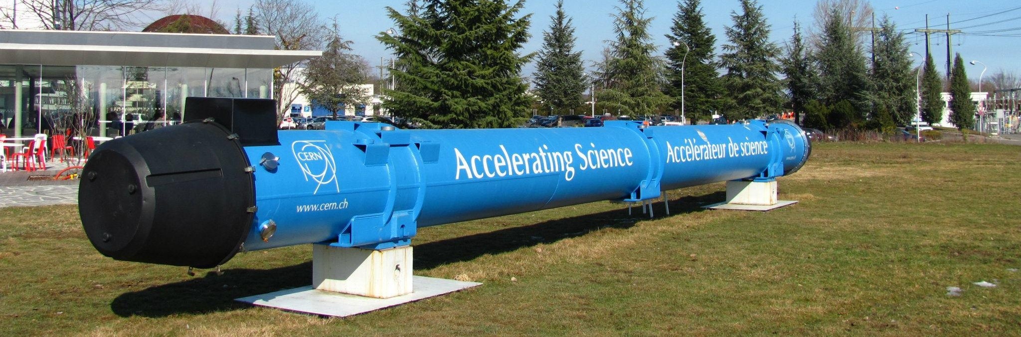
In Auger, we are interested in study the ultra high energy cosmic rays with energies above 10^17eV. To give one idea, one proton with 50EeV (5x10^19 aprox. 8 Joules) has the same energy of a tennis ball with a velocity of 60km/h. However, the tennis ball has aproximatly 6.7cm, while the proton has 0.8775x10^-13cm. In order to detect comic rays with extremely high energy, we have detector spread in a 3000km^2 in Argentina.
There are many unknowns that we want to study, like for example the end of the spectrum. At aprox. 10^20eV energy, it is expected that the cosmic ray flux be extremely supressed due to the GZK cutoff (see wiki, paperG, paperZK). However, previous experiments had contradicting results, for example, AGASA with the black diamond in the graphic, the end of the espectrum apears to be flat with no decrease in flux, while Flys Eye showed results compatible with GZK.
The recent Auger results, shows that in fact, there is a very high supression in the flux compatible with GZK.
| Global annual radiation exposure from UNSCEAR 08 Report | ||
| Type | Source | World average (mSv) |
| Natural | Radon | 0.6 |
| Ingestion | 0.29 | |
| External Terrestrial | 0.48 | |
| Cosmic | 0.39 | |
| Man made | Medical | 0.6 |
| Fallout | 0.007 | |
| others | 0.0052 | |
| Total | 3.0 | |
Sources and anisotropies
There many unknows on the cosmic rays studies, for example what are the universe structures that can produce such high energy particles? where they came from? Are cosmic rays isotropic?
We cannot forget that this particles have extremly energy. Our sun, can produce particle around 10^9eV (above the energy to do fusion), while our cosmic rays have 10^19eV energy.

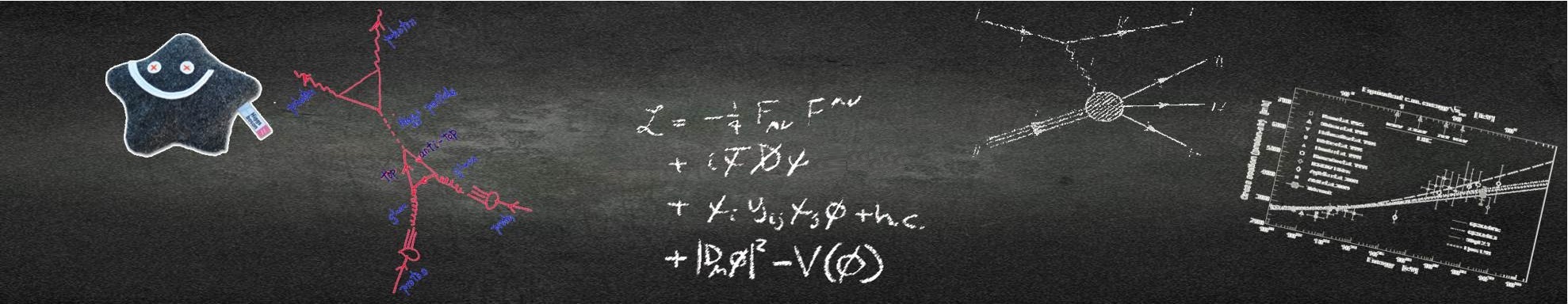
The mechanisms of acceleration of UHECR are a subject of controversy with still open questions, there are two major types of acceleration, the bottom-up and top-down.
The bottom-up mechanisms, assume that the particles are accelerated directly from low to high energies. We can have acceleration by electric Fields, although it is easy to accelerate charged particles with electric Fields, for these energies it would require a high density of particles in order to produce the field. This would cause large energy losses of the accelerated particles, making it dificult to try to reproduce the spectrum, and today it is not very accepted. Another bottom-up was proposed by Fermi in 1949, which consisted in statistical acceleration, since the particles could be accelerated each time they interact with magnetized plasma. The problem is that both models need to get a spectrum index greater than that observed to contain the energy losses of particles (for details see paper, wiki ).
Another type is the top-down model, whereby super-massive particles would decay producing UHECR. The decay of these particles would produce leptons and hadrons, the pions in turn produce muons, electrons photons and positrons. This would cause a spectrum dominated by photons at high energies. In addition the initial particle would have energies far above 10^20 and have a sufficient density to maintain the CR flux. These particles could be relics of the early universe at GUTs energies (see for example paper). Another model is the Z-burst, where UHE neutrinos interact with cosmic neutrinos background producing Z which in turn would decay into protons, neutrinos and photons. These neutrinos would come from even more energetic particles, which is difficult to explain. Besides, the flux of photons and high energy neutrinos would be very high, the current limits are major constraints in this scenario (see paper).
Propagation
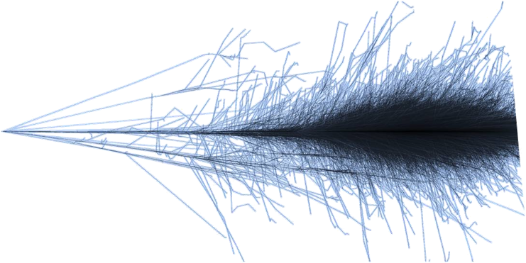
The particles (cosmic rays) that hits the Earth, have some different trajectories in space, before arrive at to us. In the bottom-right figure, we can see some particles trajectories. In the Universe, we have several structures with magnetic fields, this magnetic field causes the particles to rotate with a radius given by (in a more appropriate units):
R(pc)=10^21 E(eV)/ q(e)B(G)
This is called the Larmor radius. So, as the energy increase, the radius od the particle movement increases. If we look to the bottom-right figure, you can see the Earth, and the red line correponds to the trajectories of a 10^18eV proton, while the black point corresponds to a 10^19eV proton trajectories. The red lines, for lower energies, are very chaotic with a lot of spirals and bendings, however, for the black lines, with higher energies, the trajectories are almost straight. If we have even higher energies, the cosmic rays trajectories would be rectilinear and they will point to their respectives sources.
The galactic magnetic fields are the order of microGauss [see paper], therefore, for protons with energy of 10^19eV, and magnetic field 1microG have a Larmor radius of 10kpc, very wide in comparison with the thickness of the galaxy (0.3 kpc). For energies of 10^15 eV, the Larmor radius is about 1pc (much smaller than the galaxy). In bottom-right figure [see paper], The proton trajectories are represented for various energies, considering magnetic fields close to nanogauss (typical intergalactic value) and areas with randomly oriented field. For E = 10^20eV , the trajectories are almost rectilinear and even with realistic magnetic fields, we can do astronomy with cosmic rays. (1EeV = 10^18EeV = 0.16 Joules; 1pc = 1Parsec = 3.09x10^13 km )
, black lines to 10^19eV Protons (higher energetic).")

We saw that considering the intergalactic magnetic fields in nanogauss, protons with an energy of 100EeV have almost rectilinear trajectories and we can use them for astronomy. In bottom figure, is represented the sky map in galactic coordinates with the 69 most energetic events (with E > 55EeV ) from 1 January 2004 until 31 December 2009 [see paper]. Auger events are represented by black dots, the solid line is the PAO field of view for zenith angles smaller than 60degrees. The Blue circles with 3.1 degrees are center position of 318 AGNs from Veron-Cetty and Veron(VCV catalogue) that lie within 75 Mpc. In the map, it looks like the directions of the cosmic rays are almost isotropic, and we can not see a good match between the directions and the catalogue.
It should be noted that the extragalactic magnetic fields are still unknown and the differences between positions can be related to the existence of magnetic dipoles, quadrupoles, or other magnetic structures that deflect the particles. Currently, attempts to infer various scenarios for the magnetic structures in the nearby universe are doing based on the deflections of the CR.
Nevertheless, it seems that are some excess of events around ( an active galactic nucleus, which is one of teh closest galaxies). In the bottom-right figure, we can see a parameter describing the directions distribution. If this p=0.21, than the directions are isotropic in the sky, however the value p mesured is different from isotropy but it is not incompatible with it. And if we take out the Centaurus A excess, the anisotropy would almost disappear.
The isotropy/anisotropy make very important constrains on our view of CR ( composition, source and so on), but the result continues to be challenging to interpret.
%,
the coloured areas corresponds to 1sigma and 2sigma uncertainties, for an isotropic distribution we should have p=21.")

Extensive Air Shower (EAS)
We can not detect the Cosmic Rays directly. Remember that we have CRs fluxes of 1particle per km2 per century, and each CR would have approximately 10^-15m. This means that we would need a continue detector with huge areas to catch the particles. However, we can detect them indirectly, since the high energy CR interacts at the top of the atmosphere, producing particles, these, in turn have sufficient energy to re-produce new particles and so on, producing a cascade called Extensive air shower (EAS) (see figures below). In this way, we can detect the particles that arrive to the ground, or throughout the atmosphere (see Auger detectors on a previous section).
In EAS, the primary particle produces secondaries particles, which in turn will have interactions and decays producing more particles (and theirs energies will decrease). So the number of particles N(X) will increase until it reaches a maximum, where the energy per particle is on average equal to the ionization energy. This is known as the Xmax. The number of particles produced is equal to the number lost by ionization. From the N(X) maximum, particles are being absorbed and N(X) decreases.
Normally, we want to study the EAS to study particles interactions. In this way, the particles number profiles are not expressed in terms of high (in m) from the ground, but in atmospheric depth crossed by the EAS since the atmosphere top (in g/cm^2). So, X is the quantity of mass crossed by the shower in g/cm^2, from the top.
The cosmic rays induces a cascade of secondary particles and the electromagnetic component dissipates its energy into the atmosphere. The shower particles, mostly electrons and positrons, deposit energy in the atmosphere by ionization or excitation of air molecules. The excited nitrogen molecules, subsequently return to their ground state partially by the emission of photons near UV region, isotropically, with wavelengths between about 300 and 400 nm. This is called fluorescence light instead of scintillation light, considering the atmosphere as a scintillation calorimeter. In this way, the energy deposited measurements in the atmosphere are proportional to the primary energy, like a calorimetric energy measurement. it is also possible to detect Cherenkov and radio radiation, or maybe even coherent synchrotron radiation emitted by charged particles in the Earth magnetic field (microwave radiation). Radiation emissions can vary from the low frequency radio emission to UV fluorescence emission.
The study of the EAS can be done through two types of detection techniques. On the one hand, the secondary particles can be sampled at ground level with arrays on the ground (SD). On other hand, the emitted radiation from the shower front, as it traverses the atmosphere, can be detected (atmospheric radiation detectors). The surface arrays are detectors on the surface, detecting all particles arriving to the ground (blue cylinder in the figure below). They can be scintillator arrays and Water-Cherenkov tank arrays. The atmospheric detectors record the radiation emitted by the secondary particles through the shower development in different frequencies. As example, the fluorescence detectors, the air Cherenkov detectors, and radio and microwave antenna arrays. In the figure below, the fluorescence detectors are represented by the right telescope, the radio and microwave detection are represented in the antennas (in the middle). The Xmax detected by the telescopes in the atmosphere corresponds to the maximum of electromagnetic particles (electrons, positrons and gammas), since the fluorescence light is mainly produced by those particles.

The EAS can be divided into three components: the hadronic; the muonic, and the electromagnetic component. The hadronic component comes from the interaction of CRs or secondary particles with the molecules of the atmosphere and are mostly mesons like pions and kaons. The muonic component contains the muons and neutrinos, while the electromagnetic component have the electrons, positrons and photons. According to [29], a vertical shower of a proton with 10^19eV, at ground, has 10^11 secondary particles with energy above 90 keV and a shower core of approx. 10km. About 99% are photons, electrons and positrons, with 90% of the primary particle energy being dissipated by the electromagnetic component.
 producing pions and other hadrons. The neutral pions decay into gamma pairs, and charged pions decay into muon and muon neutrino.")

In the next part I will show some videos and pictures about the cascade development. You Should click on the images to see movies and pictures with better quality.
There are several Simulations Programs of Extensive Air Showers (EAS). We have for example, CORSIKA, CONEX, AIRES and several others. This programs simulates the particle interactions and follow them across the atmosphere. In this page the Shower animations came from CORSIKA, you can see more outputs and informations at http://www-ik.fzk.de/corsika/.
The bottom-left picture is EAS for a proton with 10^15eV with 45degrees, the Axis ranges in Z from 0 to 71.6 km and in X from -6.9 to 64.3 km. The right picture is an EAS for a vertical proton with 10^11eV.
")

The next, pictures corresponds to movies about the shower development, Click them to see the gif movies. (the gifs are not embedded to decrease the page size)
In the bottom-left, you can see a 3D perspective of an Extensive Air Shower for a vertical primary proton with 100 TeV (10^14eV).It has the particle traces of hadrons in blue, the muons in Grey, electrons in red and neutrons in green. The distances are in meters, the first interaction between the proton and the atmosphere take place at 21311m height.
In the bottom-right, is a side perspective of an EAS. The primary is a proton with 1 PeV(10^15eV) and 30 degrees. You can see the particles propagation in the sky (lateral view), each circle is a weighted particle, the same colors apply here, blue for hadrons, Grey for muons, red for electrons and green for neutrons. Note that, some particles disappear (because they are absorbed) and new ones appear in the interactions.
 and 30 degrees.")

The next, pictures corresponds to movies about the shower development, Click them to see the gif movies. (the gifs are not embedded to decrease the page size)
In the bottom-left, you can see an upwards, co-moving view of an EAS of a primery proton with 10^14eV. You can see the particle in the xy plane (like viewing the shower from above). The number of particles is increasing (in time or as we go down in the atmosphere), the total number of particles as function of height is simultanealy displayed alongside. You can also see the number of different particles as function of the radius below. The colors code is the same, blue for hadrons, Grey for muons, red for electrons and green for neutrons.
In the bottom-right, you can see a side view on an EAS of a primery proton with 10^14eV. In this case, you can see the particle in the xz plane. You can see the particles front moving in the sky, the shower is getting wider in radius as it develops and the front gets also wider, since some particles goes faster/slower getting ahead/delayed. The total number of particles as function of height is simultanealy displayed alongside. You can also see the number of different particles as function of the radius below. The colors code is the same, blue for hadrons, Grey for muons, red for electrons and green for neutrons.


Hadronic Models and Particle Physics
The characteristics of the EAS can be related with the interaction proprieties involved in the shower development. These features, like the Xmax for the electromagnetic and muonic part, the number of particles and so on, are important to try to determine the cosmic ray composition. We can only indirectly infer if the cosmic rays are protons, irons or others thing through the EAS properties. Models have been built, like EPOS, QGSJET and SYBILL to describe the high energy interactions and simulate the shower developments. Nevertheless, the firsts interactions at an Auger event are normally hadronic interaction at higher energies then the ones currently accessible in accelerators (see next section proton cross-section). These interactions are extrapolations from the accelerators data, with an high uncertainty, so it's difficult to say from the data if the results come from the composition of the cosmic rays or from differences on the interactions models at high energies.

Click in pic
OnE of the most important characteristics of the EAS used for composition and particle physics is the electromagnetic Xmax. On the right figure, the Xmax distribution from the data with 18.5 < Log En < 18.6, is drawn. If you click the image you can see all Xmax distributions from Auger. Two thing can be used to composition of physics analysis, the mean Xmax and the variation (RMS) of the Xmax evolution with energy. You can see the Xmax and RMS in the figures below.
The Xmax from proton primaries is higher of more penetrating, mainly because the proton-air cross section is lower than iron-air. This means the first interaction in the proton case, would occurs late in the atmosphere. The difference between proton and iron is around 85 g/cm^2. On our data, we found that the Xmax is close to proton at 10^18 eV, but it seems to became heavier with energy. This points out to an heavier composition, but can also indicate an increase in the proton-air cross-section at higher energies.
The fluctuation on the Xmax can also gives hints about the cosmic rays composition. Below, you can also see that the composition is compatible with proton at 10^18 eV and gets a lot heavier with energy. These two parameters are not enough to have clear picture of what's happening and we should look to another properties.


Proton Cross-section
The slope of the right tail in the Xmax distribution, at a specific energy, is proportional to the first primary cosmic particle interaction length in the atmosphere. In this way, it is possible to recover the CR inelastic cross-section with air. Assuming a proton composition, the inelastic proton-air cross-section have been reported at 57 TeV and 95 TeV at Pierre Auger Observatory and TA respectively. The Glauber formalism allows to recover the proton-proton cross-section. The results of both experiments are compatible with the models as can be seen in the figure below.


Muon content
Extensive air showers with zenith angles above 62 are dominated by secondary energetic muons at the ground since the electromagnetic component has been largely absorbed in the large atmospheric depth crossed by the shower. The SD signals of those events provide a direct measurement of the muon number on the ground. The muon number in inclined air showers is measured using the relative scale factor N19, which relates the observed muon densities at the ground to the average muon density profile of simulated proton-induced air showers of fixed energy 10^19 eV, with QGSJet01. This N19 is then corrected to the unbias Rmu. We can say that the Rmu is a measure of the muon number of the shower, that arrive on the ground. In the below figure, in the left, the evolution of the Rmu in the data is plotted. On the right, the Rmu is rescaled, for better understanding and compared with the models. In this way, most of the energy scaling is cancelled and emphasizes the effect of the cosmic-ray mass A on the muon number. The high abundance of muons in the data reflects a discrepancy between the models and the data. The measured muon number is higher than in pure iron showers, suggesting contributions of even heavier elements. This interpretation is not in agreement with studies based on the depth of shower maximum (described before). A pure proton composition would be very disfavoured with theses results, based on the hadronic models.


MPD and Muonic Xmax
It is possible to reconstruct the Muon Production Depth distribution (MPD) using the signals of the surface detectors far from the shower core. The electromagnetic signal on the SD is treated as a background, so the results are only applied for events with zenith angles in the interval [55; 65]. In inclined events, the electromagnetic signal are highly attenuated. Far from the core, the particle's arrival time is spread enough and with lower electromagnetic contamination, so using the timing information of the signals and the geometry, it is possible to reconstruct a muon production depth distribution (see figure below in the left). From MPD distributions, it is possible to obtain the muonic Xmax, as the depth along the shower axis where the production of muons reaches the maximXmax is drawn. Accordingly with the two models presented, the composition seems to become heavier and for EPOS-LHC it becomes heavier than iron. Again, the muonic Xmax show that the models have difficulty to deal with the muonic sector, which means that there are some problems describing the hadronic interactions.


Composition
For a more quantitative study of the composition evolution, using the hadronic model predictions, the Xmax and RMS(Xmax) can be converted into lnA distributions. The composition obtained from this method is drawn in the figure below for the models Sibyll2.1 , EPOS-LHC and QGSJet-II.04 . In a pure iron sample, average lnA˜4 and for proton would be average lnA˜1. In respect to the variance of lnA, a maximal mixing of 50% proton 50% iron would give V(lnA)=4 while a pure composition would give V(lnA)=0 . The composition is lightest at around 1018:3 eV and the different features of hadronic interactions implemented in the three models give rise to differences in lnA of about 0.3. The EPOS-LHC model gives the heavier interpretation of the data and in both three models, the composition is getting heavier. The variance of lnA suggests the cosmic rays are composed of different nuclei at low energies and dominated by a single type of nucleus above 10^18.7 eV, since the variance, V(lnA), is close to zero. The QGSJet-II.04 model leads to unphysical variances (V(lnA) < 0) above 10^18.4 eV and therefore this model is disfavoured by Auger data (but still within the systematics plus statistical uncertainty).

Composition and combined results
Combining observables from both electromagnetic and muonic components, the internal consistency of hadronic interaction models can be tested. It is possible to obtain the average lnA, using the muonix Xmax results in the same way as done previously for the electromagnetic part. If the hadronic models are consistent in the electromagnetic and muonic component, then the average lnA, from Xmax and muonic Xmax would overlap within the same model, despite different results between models. On the figures below, the combined results of hlnAi are drawn for Epos-LHC and QGSJet-II.04 . In the case of EPOS-LHC , the mean lnA values extracted from the Xmax and muonic Xmax are incompatible at a level of at least 2.5 sigma. With QGSJet-II.04 the lnA values are compatible, however, it should be remembered that this model has problems to describe average lnA and V(lnA) in a consistent way. None of the interaction models recently tuned to LHC data provide a consistent description of the Auger data on EM and MPD profiles.


On the below figure, in the left, the average lnRmu versus Xmax for an energy 10^19 eV is plotted. The Auger result falls completely out of the phase space allowed by the hadronic models. In the right, the slope of the evolution with energy of the value lnRmu is drawn for the data and models. In blue squares and red circles are the respective values for iron and proton showers. The white hexagon corresponds to the average lnA obtained from the electromagnetic Xmax, within each model. None of the models is covered by the total uncertainty interval. The deviation between measurement and lnA- based predictions is 1.3 to 1.4 sigmas. The large measured value of dlnRmu /d lnE disfavours a pure composition hypothesis.

Notes:
*1 Sketch of the detection principles of a fluorescence detector, from Antoine Letessier-Selvon, Todor Stanev, "Ultra high Energy Cosmic Rays", Rev. Mod. Phys, 83, 907-942 (2011); arXiv:1103.0031v1.
*2 A. Hillas, The origin of ultra-high energy cosmic rays, Annual Review of Astronomy and Astrophysics 22, p. 425-444, 2009.
*5 Arrival directions of 69 CRs with energy E>= 55 EeV detected by the Pierre Auger Observatory, from Update on the correlation of the highest energy cosmic rays with nearby extragalactic matter, Astroparticle Physics V34, I5, 2010.
6* from Anisotropy and chemical composition of ultra-high energy cosmic rays using arrival directions measured by the Pierre Auger Observatory, JCAP06(2011)022.
